
Combining data from different survey projects creates new opportunities for research, alas, at the cost of increased volume (obviously) and complexity of the data. The Survey Data Recycling project created a dataset with data from 22 international survey projects. This post shows how to access and explore this dataset, and how to select a subset for further analysis based on the availability of variables.
Introduction
More and more cross-national survey projects collect new data using better methodologies, ex ante harmonization, following higher standards, and covering more and more diverse countries. The abundance of new survey data only increases the problem of backward and parallel compatibility, because new surveys cannot be easily combined with existing survey data or data from different survey projects, which prevents analyses on a global scale.
One solution to this problem is ex post survey harmonization, i.e. combining existing data from cross-national surveys and transforming original (source) variables to a common coding scheme. The Survey Data Harmonization project and its successor, the Survey Data Recycling (SDR) project, took on the challenge of ex post harmonization of data from 22 international survey projects. The resulting dataset (Master File) contains 2,289,060 records (corresponding to individual respondents) from 142 countries/territories between 1966 and 2013. Harmonized variables include: trust in state institutions (parliament, political parties, justice system, government), political engagement (participation in demonstrations, signing petitions, interest in politics), social trust, and sociodemographics: age, gender, education, rural and metropolitan residence.
The harmonized SDR data and documentation, including detailed descriptions of the harmonization process of each target variable and recode syntax, are available on Dataverse. For more information about the SDR project, including the project team, funding sources, the source data, a description of the SDR idea, publications and conference presentations, see the project website dataharmonization.org.
The clear advantage of SDR data is its extended coverage, both geographically and over time. The cost of this is increased volume and complexity. In this post I show how to download and explore the individual-level dataset (Master File).
Survey projects in SDR v.1:
| Abbr. | Project name |
|---|---|
| ABS | Asian Barometer |
| AFB | Afrobarometer |
| AMB | Americas Barometer |
| ARB | Arab Barometer |
| ASES | Asia Europe Survey |
| CB | Caucasus Barometer |
| CDCEE | Consolidation of Democracy in Central-Eastern Europe |
| CNEP | Comparative National Elections Project* |
| EB | Eurobarometer* |
| EQLS | European Quality of Life Survey |
| ESS | European Social Survey |
| EVS | European Values Study |
| ISJP | International Social Justice Project |
| ISSP | International Social Survey Programme* |
| LB | Latinobarometro |
| LITS | Life in Transition Survey |
| NBB | New Baltic Barometer |
| PA2 | Political Action II |
| PA8NS | Political Action - An 8 Nation Study |
| PPE7N | Political Participation and Equality in 7 Nations |
| VPCPCE | Values and Political Change in Postcommunist Europe |
| WVS | World Values Survey |
| *Selected waves or samples. | |
| Note: Data as of Q2 2014. |
Downloading the SDR data
The SDR data bundle version 1 (Master Box v.1) is available from Dataverse. Thanks to the dataverse package, these data can be loaded directly to R.
Here are all the other necessary packages:
library(dataverse) # to access data from Dataverse
library(tidyverse) # to clean and reshape the data
library(rijkspalette) # to get pretty colors for the graphs
library(knitr) # to create nice tables
library(kableExtra) # to customize tables (kables)
library(sf) # to encode spatial vector data for maps
library(countrycode) # switch between country codes
Knowing the repository’s DOI, one can get a list of all data and documentation file with the get_dataset function1.
get_dataset("doi:10.7910/DVN/VWGF5Q") # lists the files from a Dataverse by its DOI## Dataset (140655):
## Version: 1.1, RELEASED
## Release Date: 2018-08-22T14:31:37Z
## License: CC0
## 21 Files:
## label version id
## 1 Merge_Files_to_Master_Box_1_0.do 2 3006242
## 2 Merge_Files_to_Master_Box_1_0.sps 2 3006243
## 3 SDR_Master_Box_Description_1_0.pdf 2 3006218
## 4 SDR_Master_File_1_0-1.tab 2 3006271
## 5 SDR_Master_File_1_0.tab 2 3006244
## 6 SDR_Master_File_Documentation_1_0.pdf 2 3006219
## 7 SDR_Master_File_SQL_Code_1_0.txt 2 3006220
## 8 SDR_Master_File_Variable_Report_AGE_1_0.tab 2 3006221
## 9 SDR_Master_File_Variable_Report_EDU_1_0.tab 2 3006222
...Among the files in the SDR Master Box there is the Master File with harmonized individual-level survey variables.2
I will use the Stata version of the SDR Master File, which has the id 3006244 (the Master File is also available in SPSS format, with the id 3006271).
The get_file function downloads the data file to R (see documentation for details). The data file is pretty large, so this may take a while.
master.raw <- get_file(3006244) # downloading the dataset by its identifier
tmp <- tempfile(fileext = ".dta")
writeBin(as.vector(master.raw), tmp)
master <- haven::read_dta(tmp) # creating a data frame from the temp file
Exploring SDR: availability of variables by project
The SDR dataset contains data from 22 projects identified by the variable t_survey_name. Each project has one or more waves (t_survey_edition), each with many national samples identified as a combination of t_survey_name, t_survey_edition, t_country_l1u, t_country_set, where t_country_set is used to distinguish national samples carried out in the same project wave (a very rare situation).
The first step of working with the SDR data is to check how many projects have variables necessary for a given analysis. Let’s say I’m interested in analyzing determinants of participation in demonstrations, and for an exploratory analysis I want to take a look at all relevant variables3:
* participation in demonstrations (t_pr_demonst_fact),
* trust in parliament (t_tr_parli_11),
* social trust (t_tr_personal),
* interest in politics (t_int_polit_5),
* education (either completed levels, t_edu, or years of schooling, t_school_yrs),
* rural residence (t_ruralurb),
* age (t_age),
* gender (t_gender).
This information can be obtained by transforming the Master File into a project-level file with the availability of the selected variables in separate columns.
The below piece of code does the following:
- lists all variable names and stores your selection as a vector (
selected_vars), - selects a subset of
masterwith only the chosen variables, - splits
masterinto groups - national surveys (identified ast_survey_name,t_survey_edition,t_country_l1u, andt_country_set), - calculates means of all numeric variables by group,
- for numeric variables, constructs a group-level logical variable, which is
TRUEwhen the mean of the given variable is not missing, andFALSEotherwise, - groups by project (
t_survey_name), - for each project, calculates the proportion of surveys that contain a given variable (proportion of
TRUEvalues), - drops unnecessary variables.
names(master)
selected_vars <- c("t_survey_name", "t_survey_edition", "t_country_l1u",
                   "t_country_set", "t_gender", "t_age", "t_edu", "t_school_yrs",
                   "t_ruralurb", "t_tr_parli_11", "t_tr_personal",
                   "t_pr_demonst_fact", "t_int_polit_5")

master_vars_survey <- master %>%
  select(selected_vars) %>%
  mutate(educ = ifelse(is.na(t_edu) & is.na(t_school_yrs), NA, 1)) %>%
  group_by(t_survey_name, t_survey_edition, t_country_l1u, t_country_set) %>%
  summarise_all(funs(if(is.numeric(.)) mean(., na.rm = TRUE) else first(.))) %>%
  mutate_all(funs(if(is.numeric(.)) as.numeric(!is.na(.)) else .)) %>%
  group_by(t_survey_name) %>%
  summarise_all(funs(if(is.numeric(.)) mean(., na.rm = TRUE) else first(.))) %>%
  select(-c("t_survey_edition", "t_country_l1u", "t_country_set",
            "t_school_yrs", "t_edu"))
The result of these operations is a data frame with 22 rows (corresponding to 22 survey projects in SDR v.1). The first column contains project names, and the next 8 columns contain values ranging from 0 to 1, corresponding to the proportion of national surveys in the given project that contain a given variable.
head(master_vars_survey)## # A tibble: 6 x 9
## t_survey_name t_gender t_age t_ruralurb t_tr_parli_11 t_tr_personal
## <chr> <dbl> <dbl> <dbl> <dbl> <dbl>
## 1 ABS 1 1 1 1 1
## 2 AFB 1 1 1 0.818 0.424
## 3 AMB 1 0.989 0.957 1 0.25
## 4 ARB 1 1 0.625 0.812 1
## 5 ASES 1 1 0.944 0.944 0
## 6 CB 1 1 1 1 1
## # ... with 3 more variables: t_pr_demonst_fact <dbl>, t_int_polit_5 <dbl>,
## # educ <dbl>Before plotting these data, it’s necessary to do a few more things:
1. convert the table to a data frame to avoid future problems,
2. use project names as row names,
3. drop the t_survey_name column,
4. assign column names,
5. convert to matrix and transpose (so that variables are in rows and projects in columns).
master_vars_survey <- master_vars_survey[, c(1,2,3,9,4,5,6,7,8)] # change the order of variables

master_vars_survey <- as.data.frame(master_vars_survey) # convert to data frame
row.names(master_vars_survey) <- master_vars_survey$t_survey_name # first variable as row names
master_vars_survey <- master_vars_survey[,2:ncol(master_vars_survey)] # drop the first variable

names(master_vars_survey) <- c("Gender", "Age", "Education", "Rural", "Trust in parliament",
                               "Social trust", "Participation in demonstrations",
                               "Interest in politics")

master_matrix <- data.matrix(master_vars_survey) # convert to matrix
master_matrix <- t(master_matrix) # transpose
Now the master_matrix is ready for plotting. First, I create a color palette from white (= no surveys in a project have the variable of interest) to sea green (= all surveys in the project have the variable of interest; the color is taken from Karel Appel’s Square man via the rijksPalette package).
Next, I set the parameters and draw the heatmap (a colored table, really).
appel <- rijksPalette("Karel Appel")
colfunc <- colorRampPalette(c("white", appel$palette(10)[7]))

x = 1:ncol(master_matrix)
y = 1:nrow(master_matrix)
centers <- expand.grid(y,x)

par(mar = c(3,15,4,2))

image(x, y, t(master_matrix),
      xaxt = 'n',
      yaxt = 'n',
      xlab = '',
      ylab = '',
      axes = FALSE,
      ylim = c(max(y) + 0.5, min(y) - 0.5),
      col = colfunc(10))

mtext(attributes(master_matrix)$dimnames[[2]],
      at=1:ncol(master_matrix),
      adj = 0, padj = 0, las=2)
mtext(attributes(master_matrix)$dimnames[[1]],
      at=1:nrow(master_matrix), side = 2, las = 1, adj = 1.02)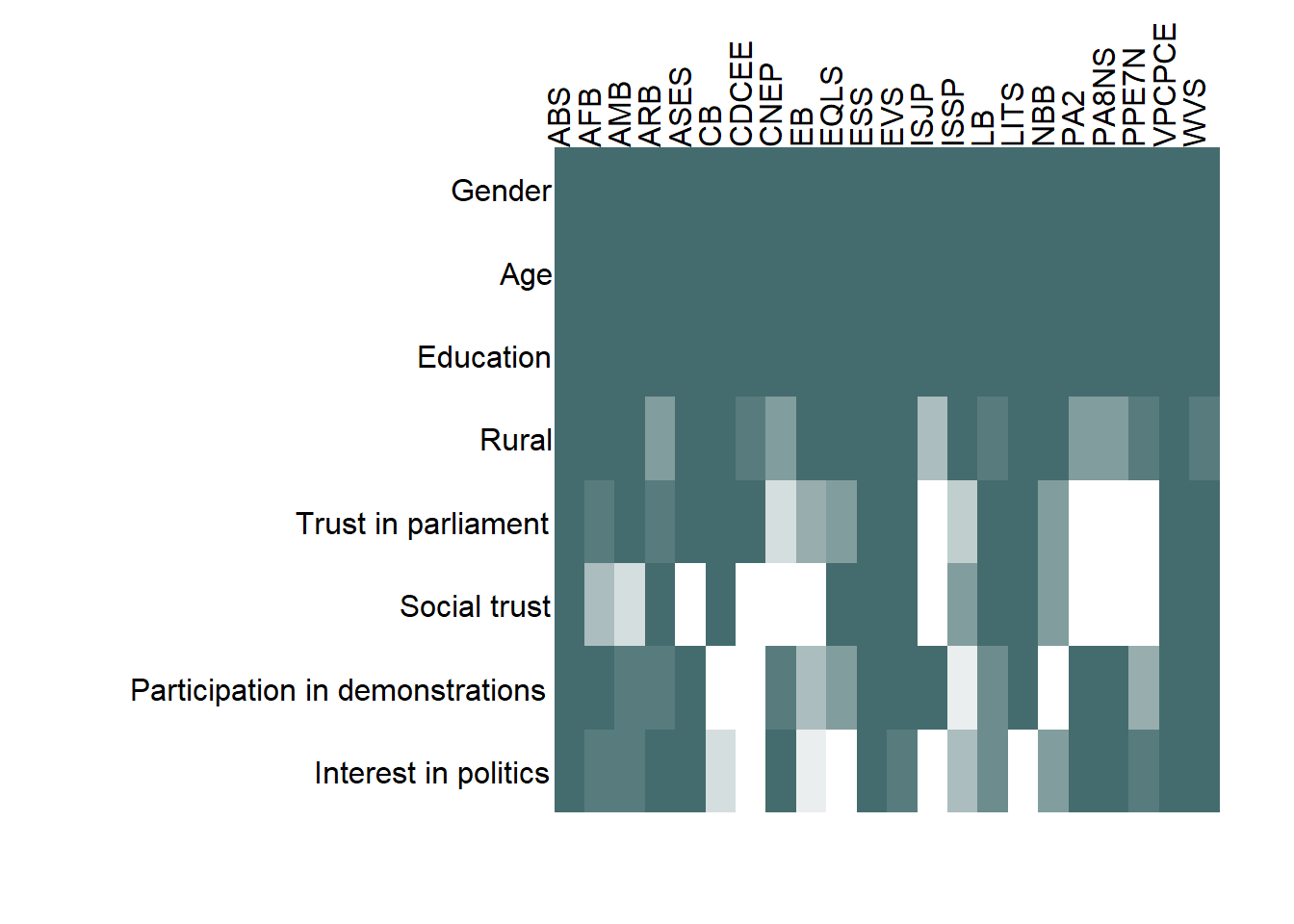
The chart shows that gender, age, and education (measured either with completed levels or schooling years) are available across projects, with only few exceptions - too few to be visible on the heatmap. The rural residence indicator is present in at least some surveys in all projects.
The availability of other variables is mixed. Trust in parliament is missing in ISJP (selected waves), PA2, PA8NS, and PPE7N. Social trust is additionally missing in ASES, CDCEE, CNEP, and EB (selected waves). The question about participation in demonstrations is asked in at least some surveys in all projects except for CB, CDCEE, and NBB.
As the next section shows, this table conceals some important heterogeneity with regard to the participation in demonstration questions.
Exploring SDR: availability of variables with different formulations
In addition to harmonizing the original (source) variables, the SDR project records various characteristics of original questionnaire items. In the SDR data these item characteristics are called harmonization controls and accompany the harmonized target variables in the Master File.
These harmonization controls capture properties of source items that might have an effect on respondents’ answers, and were selected following a review of the relevant methodological literature and of the original questionnaires of the harmonized surveys. These include, for example, the length of the original response scales in questions about trust in state institutions, or whether the information about rural/urban residence was provided by the respondent or coded by the interviewer.
Some of the properties captured with harmonization controls influence the distribution of responses more than others. One of the properties with a direct effect on response is the time-frame in the question about protest participation, for example participation in demonstrations. Some surveys ask about participation “last year” or “in the last 12 months”, others about the last 2, 3, 4, 5, 8 or 10 years, and some do not specify a time frame, i.e., ask about participation “ever”. Logically, the proportion of individuals who participated in a demonstration “ever” is higher than of those who participated “last year”. These two groups might also be different in other ways. Combining surveys with different question formulations might yield misleading results, especially in analyses modeling the sample proportion of participation in demonstrations.
When analyzing, for example, determinants of participation in demonstrations, it could be a good idea to decide a priori which type of questions to focus on. Again, the first step would be to see how frequently these different formulations occur in survey projects. In the SDR dataset the number of years in the original (source) question on participation in demonstrations is preserved in the control variable c_pr_demonst_years.
Doing this requires a few modifications to the data preparation code used in the previous example. I also narrow down the selection of variables in selected_vars_2.
selected_vars_2 <- c("t_survey_name", "t_survey_edition", "t_country_l1u", "t_country_set",
                   "t_gender", "t_age", "t_edu", "t_school_yrs", "t_ruralurb",
                   "t_tr_parli_11", "t_pr_demonst_fact", "c_pr_demonst_years")

master_vars_survey_2 <- master %>%
  select(t_case_id, selected_vars_2) %>%
  mutate(educ = ifelse(is.na(t_edu) & is.na(t_school_yrs), NA, 1)) %>%
  spread(c_pr_demonst_years, t_pr_demonst_fact) %>%
  group_by(t_survey_name, t_survey_edition, t_country_l1u, t_country_set) %>%
  summarise_all(funs(if(is.numeric(.)) mean(., na.rm = TRUE) else first(.))) %>%
  mutate_all(funs(if(is.numeric(.)) as.numeric(!is.na(.)) else .)) %>%
  group_by(t_survey_name) %>%
  summarise_all(funs(if(is.numeric(.)) mean(., na.rm = TRUE) else first(.))) %>%
  select(-c("t_survey_edition", "t_case_id", "t_country_l1u", "t_country_set",
            "t_school_yrs", "t_edu"), -ncol(.)) %>%
  select(1,2,3,6,4,5,7,8,9,10,11,12,13,14)
After the data are prepared, the remaining steps are the same.
master_vars_survey_2 <- as.data.frame(master_vars_survey_2)
row.names(master_vars_survey_2) <- master_vars_survey_2$t_survey_name
master_vars_survey_2 <- master_vars_survey_2[,2:ncol(master_vars_survey_2)]


names(master_vars_survey_2) <- c("Gender", "Age", "Education", "Rural", "Trust in parliament",
                               "Demonstrations (1 year)", "Demonstrations (2 years)",
                               "Demonstrations (3 years)", "Demonstrations (4 years)",
                               "Demonstrations (5 years)", "Demonstrations (8 years)",
                               "Demonstrations (10 years)", "Demonstrations (ever)")

master_matrix_2 <- data.matrix(master_vars_survey_2)
master_matrix_2 <- t(master_matrix_2)

x = 1:ncol(master_matrix_2)
y = 1:nrow(master_matrix_2)
centers <- expand.grid(y,x)

par(mar = c(3,13,5,2))

colfunc <- colorRampPalette(c("white", appel$palette(1)[1]))

image(x, y, t(master_matrix_2),
      xaxt = 'n',
      yaxt = 'n',
      xlab = '',
      ylab = '',
      axes = FALSE,
      ylim = c(max(y) + 0.5, min(y) - 0.5),
      col =  colfunc(10))

mtext(attributes(master_matrix_2)$dimnames[[2]],
      at=1:ncol(master_matrix_2),
      adj = 0, padj = 0, las=2, cex = 1.2)
mtext(attributes(master_matrix_2)$dimnames[[1]],
      at=1:nrow(master_matrix_2), side = 2, las = 1, adj = 1.02, cex = 1.2)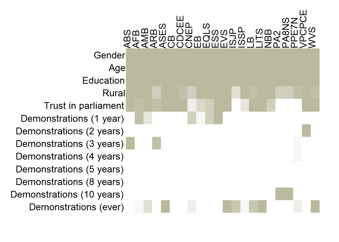
This second heatmap reveals considerable variation in the design of the “participation in demonstrations” questions across survey projects. Although almost all projects contain some variant of this question, in most projects it’s either the “last year” or “ever” variant. Other versions are rare and available in a single project or in only few projects.
Identifying surveys containing selected variables
Finally, in order to select the right subset of the SDR Master File, it’s necessary to know which surveys have all the variables of interest. Let’s assume I’m still interested in analyzing trust in parliament, education, and participation in demonstrations, but this time I only take surveys where questions about participation in demonstrations do not contain any time specification, i.e., “ever” (c_pr_demonst_years == 11). I add t_case_id to the selected variables to uniquely identify rows for spreading.
selected_vars_3 <- c("t_country_set",
                     "t_case_id", "t_survey_name", "t_survey_edition", "t_country_l1u",
                     "t_gender", "t_age", "t_edu", "t_school_yrs", "t_ruralurb",
                     "t_tr_parli_11", "t_pr_demonst_fact", "c_pr_demonst_years")

surveys_with_vars <- master %>%
  select(selected_vars_3) %>%
  mutate(educ = ifelse(is.na(t_edu) & is.na(t_school_yrs), NA, 1)) %>%
  spread(c_pr_demonst_years, t_pr_demonst_fact) %>%
  group_by(t_survey_name, t_survey_edition, t_country_l1u, t_country_set) %>%
  summarise_all(funs(if(is.numeric(.)) mean(., na.rm = TRUE) else first(.))) %>%
  select(t_survey_name, t_survey_edition, t_country_l1u, t_country_set, t_gender,
         t_age, t_ruralurb, t_tr_parli_11, educ, demo11 = "11") %>%
  filter_at(vars(t_gender, t_age, t_ruralurb, educ, t_tr_parli_11, demo11),
            all_vars(!is.na(.))) %>%
  select(t_survey_name, t_survey_edition, t_country_l1u, t_country_set)

nrow(surveys_with_vars)
## [1] 557The result is a data frame with rows corresponding to national surveys and four variables that uniquely identify a national survey: t_survey_name, t_survey_edition, t_country_l1u, t_country_set. The first six rows look like this:
kable(surveys_with_vars[1:6,], align=c("c", "c", "c", "c")) %>%
  kable_styling(full_width = F, position = "left") %>%
column_spec(1:4, width = "10em")| t_survey_name | t_survey_edition | t_country_l1u | t_country_set |
|---|---|---|---|
| AMB | 2004 | BO | 1 |
| AMB | 2004 | CO | 1 |
| AMB | 2004 | CR | 1 |
| AMB | 2004 | GT | 1 |
| AMB | 2004 | HN | 1 |
| AMB | 2004 | MX | 1 |
The 557 selected national surveys come from 7 survey projects as listed below.
surveys_with_vars %>% group_by(t_survey_name) %>% count() %>%
  kable(., col.names = c("Project", "N surveys"), align=c("c", "c")) %>%
  kable_styling(full_width = F, position = "left") %>%
column_spec(1:2, width = "10em")| Project | N surveys |
|---|---|
| AMB | 34 |
| ASES | 16 |
| EVS | 121 |
| ISSP | 37 |
| LB | 145 |
| LITS | 62 |
| WVS | 142 |
Subsetting the Master File
Knowing the key variables identifying national surveys with all the variables of interest (stored in surveys_with_vars), an inner_join will generate the appropriate subset of the Master File. The subset contains data from 557 national surveys from 7 survey projects, carried out in 111 countries/territories between 1981 and 2010, with a total of 702707 respondents. Further analyses can be performed on this subset only.
master_select <- inner_join(master, surveys_with_vars,
                            by= c("t_survey_name", "t_survey_edition",
                                  "t_country_l1u", "t_country_set"))

master_select %>%
  mutate(survey = paste(t_survey_name,t_survey_edition,t_country_l1u,t_country_set,sep = "")) %>%
  summarise(min(t_country_year), max(t_country_year),
            length(unique(t_country_l1u)),
            length(unique(t_survey_name)),
            length(unique(survey)),
            n()) %>%
  kable(., col.names = c("Min year","Max year","N countries","N projects",
                         "N surveys","N individuals"),
        align=c("c","c","c","c","c","c")) %>%
  kable_styling(position = "left") %>%
column_spec(1:6, width = "7em")| Min year | Max year | N countries | N projects | N surveys | N individuals |
|---|---|---|---|---|---|
| 1981 | 2010 | 111 | 7 | 557 | 702707 |
Country coverage plot
The last thing I will do is to plot the country coverage of the Master File subset on the world map. As a reminder, this subset contains all surveys from the SDR Master File that have all of the following variables: gender, age, education (completed levels or schooling years), rural residence, trust in parliament, and participation in demonstrations “ever”.
There are a few ways of doing this, one of which uses the rworldmap package. A small fix is necessary to deal with Kosovo, which has no ISO2 code assigned in the rworldmap data, but does have an ISO3 code (KOS). The SDR data use ISO2 codes, so it’s necessary to convert them to ISO3 (with just one line of code thanks to the countrycode package!).
# data frame with unique country codes
countries <- data.frame(iso2 = unique(substr(surveys_with_vars$t_country_l1u, 1, 2)),
  stringsAsFactors = FALSE) %>% mutate(n = 1)

world <- st_as_sf(rnaturalearth::countries110)
  world$iso_a2[world$sovereignt == "Kosovo"] <- "KS"
  world <- world[world$name != 'Antarctica',]

merge <- left_join(world, countries, by = c("iso_a2" = "iso2"))

ggplot(merge, aes(fill=factor(n))) +
  geom_sf(alpha=0.8,col='white') +
  coord_sf(crs = "+proj=moll") +
  ggtitle('Country coverage: trust in parliament and demonstrating "ever"') +
  labs(caption="Source: SDR v.1") +
  scale_fill_manual(na.value = "transparent",
                      values = "deepskyblue4") +
theme(legend.position = "none") 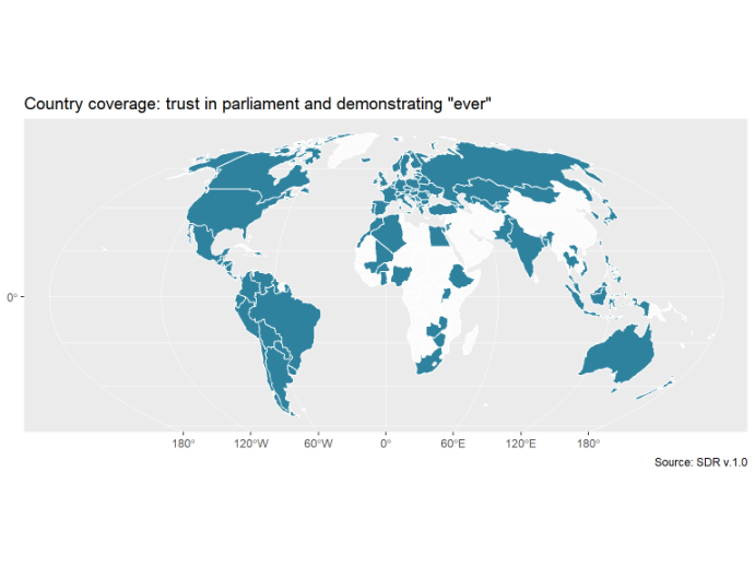

In order to show only a snippet of the long output I used a custom output hook function with
knitrfound on StackOverflow.↩Other data files contain variables measured at different levels:
SDR_Plug_Country_Year_1_0has country-year-level variables like GDP per capita or measures of democracy;SDR_Plug_Survey_1_0has quality indicators and methodological variables at the level of the national survey;SDR_Plug_Wave_1_0has quality indicators for project waves, andSDR_Plug_Country_1_0has country and continent codes.↩Note that some variables are available in different versions, i.e., one version of trust in state institutions has been rescaled to 0-10, another to 0-1, and the third version records the relative position in the sample distribution. For more information on the different variants of harmonized variables see the SDR documentation on Dataverse.↩